Hey guys, this is not an article I wrote but was written by a friend of mine. They gave me permission to add their article to my site and if you’d like to see the original read, it can be found on Medium in this article. Thanks and I hope you browser the other readings!
Understanding the data, logistic regression, random forest, confusion matrix, and grid search cv.
By Justin Behringer
Introduction:
For this month I have learned a lot about different models and hyperparameters. Today we will be looking at the difference between Linear and Classification models on a data frame to predict the price range of a cell phone. We will see the models being built, their performances, and how to improve the models by using hyperparameters on them. Everything you will see today will be mainly on python, NumPy, and sklearn.
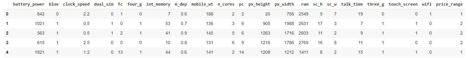
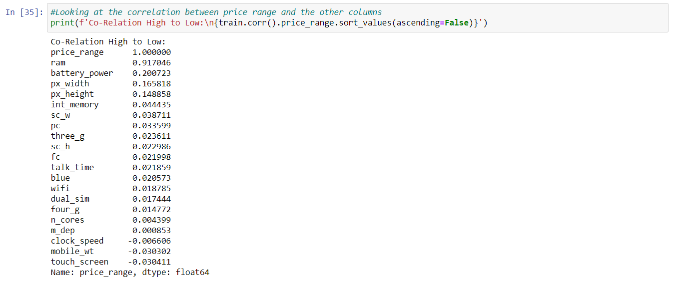
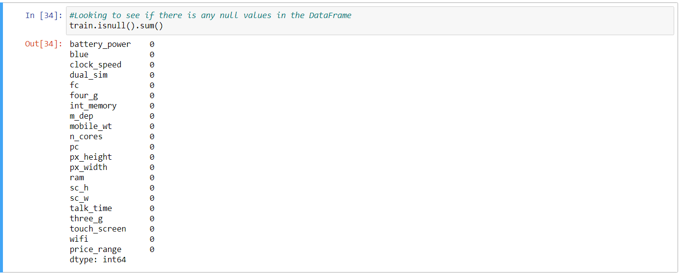
I am using a dataset that was found on Kaggle to predict the price range of cell phones based on the features for the phone. The first thing I did was load in the data frame and check for NaN values and check the correlation between price range in the data frame.
Here is the data dictionary so we can see and understand exactly what each column represents.
- battery_power = Total energy a battery can store in one time measured in mAh.
- blue = Has Bluetooth or not. | 1: Has, 0: Does not have.
- clock_speed = Speed at which microprocessor executes instructions.
- dual_sim = Has dual sim support or not | 1: support, 0: Does not support.
- fc = Front Camera megapixels.
- four_g = Has 4G or not. | 1: Has, 0: Does not have.
- int_memory = Internal memory in gigabytes.
- m_dep = Mobile Depth in cm.
- mobile_wt = Weight of mobile phone.
- n_cores = Number of cores of the processor.
- pc = Primary Camera megapixels.
- px_height = Pixel Resolution Height.
- px_width = Pixel Resolution Width.
- ram = Random Access Memory in MegaBytes.
- sc_h = Screen Height of mobile in cm.
- sc_w = Screen Width of mobile in cm.
- talk_time = Longest time that a single battery charge will last when you are.
- three_g = Has 3G or not. | 1: Has, 0:Does not have.
- touch_screen = Has touch screen or not. | 1: Has, 0:Does not have.
- wifi = Has wifi or not. | 1:Has, 0:Does not have.
- price_range = This is the target variable. | 3:Very High Cost, 2:High Cost, 1:Medium Cost, 0:Low Cost.
Data visualization:
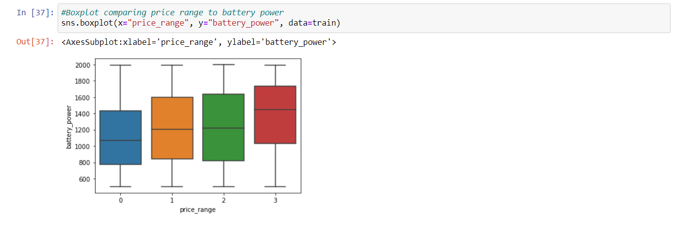
I then made a boxplot showing the comparison between price range and battery_power. As you can see from the graph below there is some comparison between price range and battery power.
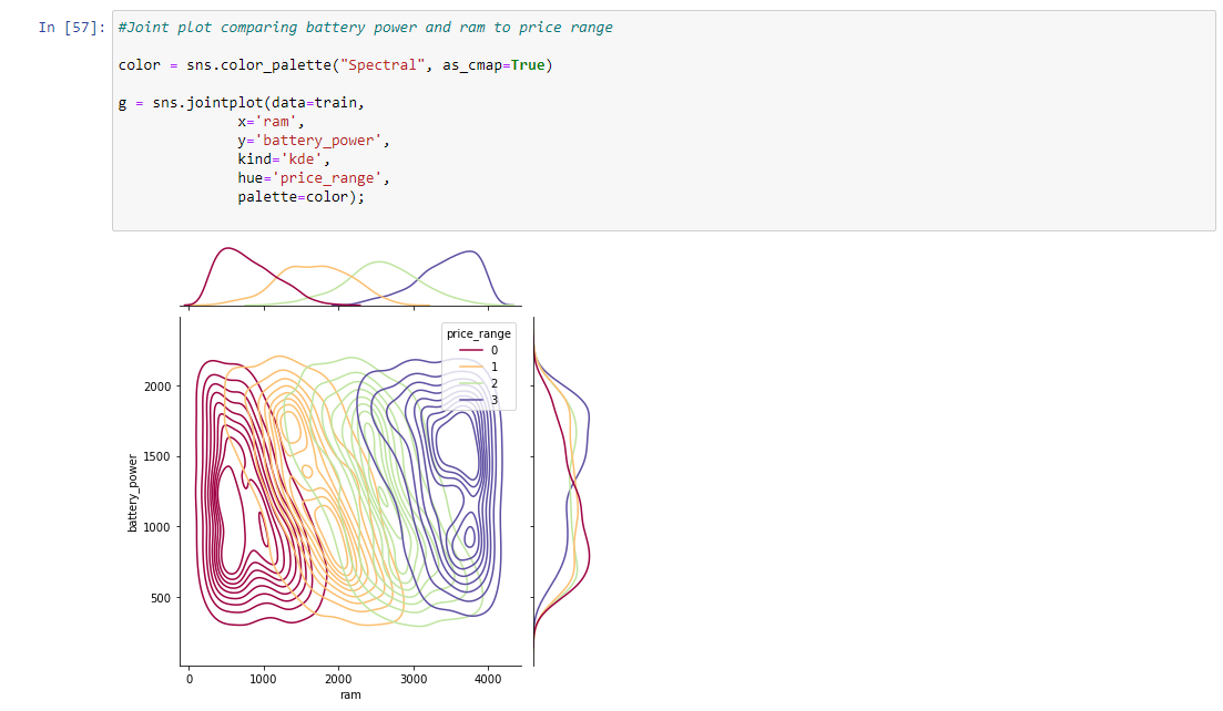
Since we saw a huge correlation between ram and price range we decided to make myself a joint plot. we used my X as ram and my Y as battery power. we then put my hue as price range to see if both of them greatly impact the cell phone price. You can see a huge impact with ram to price range from the graph below.
Splitting data into testing and validation sets:
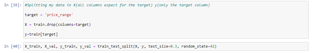
After making sure my data frame looked correct I started splitting the data up. Since there is already a test CSV file, we decided to split the training data frame into train and validation sets. I used 30% for the validation since this was a small data frame. In the end, the training set had 1400 rows and the validation set had 600 rows.
Linear regression:
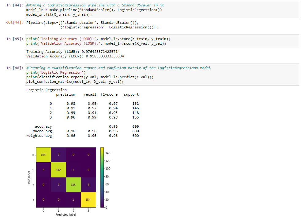
For the first model, I used a standard scaler to scale are data variance and logistic regression. We then fit the X_train and Y_train to the first model. When you look at the accuracy score for training and validation in the model we can see a lot of overfitting. This can be from data leaking in the data frame. I also looked at a classification report and plotted a confusion matrix.
Since we have all the necessary metrics for low cost from the confusion matrix, now we can calculate the performance measures for low cost. For example, class low cost has:
- 0.96 is the precision score for low cost. 144/(144 + 7) is how we got the precision score
- 0.97 is the recall score for low cost. 144/(144 + 4) is how we got the recall score.
- 0.48 is the F1–score for low cost. (.96 * .97)/(.96 + .97) is how we got the F1 score for low cost.
Random forest classifier:
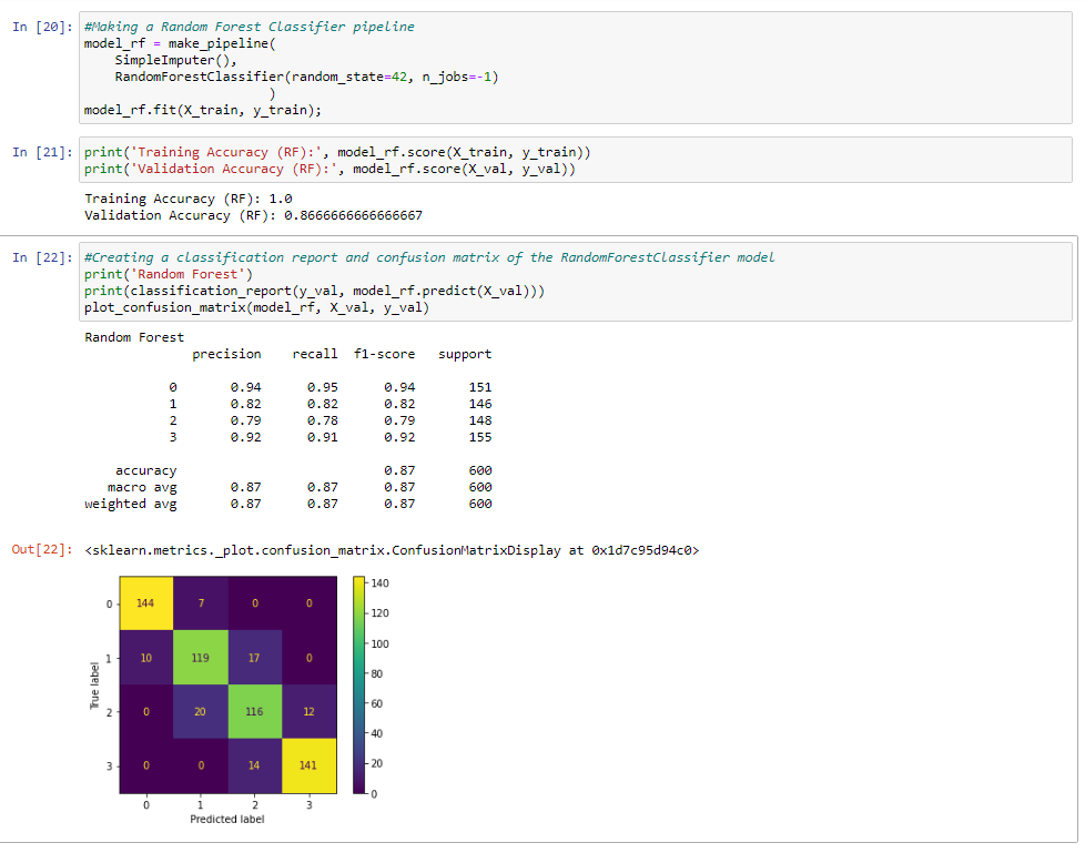
In the second model, I used a standard scaler and random forest classifier. We set the random state to 42 and are n jobs to -1. When we look at the accuracy score we can find a 1 for the training set and a .86 for the accuracy score.
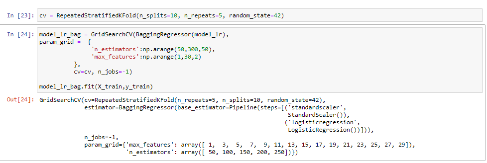
We are now going to start tuning our logistic regression model since it had the best results. I will be using a grid search cv and putting our model in a bagging regressor. We are using the bagging regressor to hopefully help with the overfitting. For the parameters, we choose to be somewhat simple. We are figuring out are best n estimators and max features for the model to help improve it.
We found that 19 was the best for max features and 150 for n estimators.
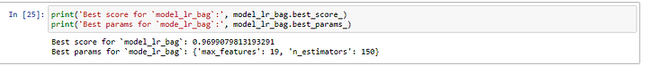
The results for the training accuracy were a little bit lower than the score but we did improve our validation accuracy by 0.16.

Conclusion:
In conclusion, the study presented in this article aimed to predict the prices of smartphones using technical specifications and machine learning algorithms. The results showed that both Random Forest and Logistic Regression models can be used to accurately predict smartphone prices based on their technical specifications.
The study found that the most important features for predicting the price of a smartphone were the display size, internal memory, RAM, and battery capacity. Additionally, it was observed that the Random Forest model outperformed the Logistic Regression model in terms of accuracy and performance.
Overall, this study demonstrated the potential of using machine learning algorithms to predict smartphone prices based on their technical specifications. The findings could be useful for smartphone manufacturers, retailers, and consumers in making informed decisions about pricing and purchasing smartphones.